Chapter 7 Lab 7
Lab 7 and 8 introduce the students to probability. In lab 7, we introduce binomial probability and then in lab 8 we introduce normal distribution probability. Again, we use an informal video by the course lead to suppport students in understanding the theoretical concepts behind probability.
7.1 Pre-class activities
7.1.1 Activity 1: Video
Watch the video on probability made by Heather where she talks through why learning about probability is relevant and how to calculate probabilities of events.
7.1.2 Probability and Probability Distributions
The aim of Lab 7 is to introduce concepts and R/RStudio functions that you can use to:
- calculate probabilities
- create probability distributions
- make estimations from probability distributions.
7.1.3 Activity 2: library
There are no cheatsheets for this lab as we will not be using a specific package. However, you can make full use of the R help function (e.g. ?sample) when you are not clear on what a function does. There are loads of videos and help pages out there with clear examples to explain difficult concepts. For now though, and to start this prep, open a new script and load in the tidyverse package (we need this for some visualisation work later).
7.1.4 Types of data
How you tackle probability depends on the type of data/variables you are working with (i.e. discrete or continuous). This is also referred to as Level of Measurements.
Discrete data can only take integer values (whole numbers). For example, the number of participants in an experiment would be discrete - we can’t have half a participant! Discrete variables can also be further broken down into nominal and ordinal variables. Ordinal data is a set of ordered categories; you know which is the top/best and which is the worst/lowest, but not the difference between categories. For example, you could ask participants to rate the attractiveness of different faces based on a 5-item Likert scale (very unattractive, unattractive, neutral, attractive, very attractive). You know that very attractive is better than attractive but we can’t say for certain that the difference between neutral and attractive is the same size as the distance between very unattractive and unattractive. Nominal data is also based on a set of categories but the ordering doesn’t matter (e.g. left or right handed). Nominal is sometimes simply refered to as categorical data.
Continuous data on the other hand can take any value. For example, we can measure age on a continuous scale (e.g. we can have an age of 26.55 years), other examples include reaction time or the distance you travel to university every day. Continuous data can be broken down into interval or ratio data; but more of that another time.
7.1.5 Simple probability calculations
Today, we are going to cover the concepts of probability calculations.
Probability is the extent to which an event is likely to occur and is represented by a real number p between 0 and 1. For example, the probability of flipping a coin and it landing on ‘tails’ most people would say is estimated at p = .5. Calculating the probability of any discrete event occuring can be formulated as:
\[p = \frac{number \ of \ ways \ the \ event \ could \ arise}{number \ of \ possible \ outcomes}\] For example, what is the probability of randomly drawing your name out of a hat of 12 names where one name is definitely yours?
## [1] 0.08333333The probability is .08, or to put it another way, there is an 8.3% chance that you would pull your name out of the hat.
7.1.6 Joint probability
Describing the probability of single events, such as a coin flip or rolling a six is easy, but more often than not we are interested in the probability of a collection of events, such as the number of heads out of 10 flips or the number of sixes in 100 rolls. For simplicity, let’s take the example of a coin flip.
Let’s say we flip a coin four times. Assuming the coin is fair (probability of heads = .5), we can ask question such as: what is the probability that we get heads on exactly one out of the four coin flips?
7.1.7 Activity 3: Estimate the probability of getting X heads over four independent flips.
Let’s start by introducing the sample() function in R, which samples elements from a vector, “x”. A vector is a sequence of data elements of the same basic type. Members in a vector are officially called components. Let’s define a vector using c("HEADS", "TAILS") and take four samples from it.
# Notice that because our event labels are strings (text),
# we need to enter them into the function as a vector; i.e. in "quotes"
sample(x = c("HEADS", "TAILS"), size = 4, replace = TRUE)
## [1] "TAILS" "TAILS" "TAILS" "TAILS"What you have done here is tell R that you want to sample observations from a set of data, which in this case was our vector c("HEADS", "TAILS"). size tells R the number of samples you want to take. We chose four, which is larger than the size of the vector itself (it has only two components; HEADS and TAILS). For this reason we need to override the default setting, which is sampling without replacement. Sampling without replacement means that once an observation appears in the sample, it is removed from the source vector so that it can’t be drawn again. Sampling with replacement means that an observation is retained so it can be drawn again. In this case, if we don’t override the default it would mean that if we tossed HEADS we wouldn’t be able to toss the coin and get HEADS again and we would get an error message because we’ve asked for more observations than are possible (we override this by setting replace to TRUE)
It will make our lives easier if we define heads as one and tails as zero and write the same command as follows:
# Now that our event labels are numeric, we don't need the combine function `c`
# 0:1 means all numbers from 0 to 1 in steps of 1. So basically, 0 and 1.
sample(0:1, 4, TRUE)
## [1] 1 1 1 17.1.8 Activity 4: sum
This is logically equivalent, but using ones and zeroes means that we can count the number of heads by simply summing up the values in the vector. For instance:
# The above statement pipes the output of sample()
#then the function sum() which counts up the number of heads.

sample(0:1, 4, TRUE) %>% sum()
## [1] 1Run this function multiple times (you can use the up arrow in the console to avoid having to type it over and over). I ran it five times the results of my little (N = 5) simulation of flipping four coins and counting heads were: 1, 3, 2, 2, and 3. So in only one out of the five simulations did I get exactly one heads.
7.1.9 Activity 5: replicate 1
Let’s repeat the experiment a whole bunch more times. We can have R do this over and over again using the replicate() function from base R. The basic syntax of replicate() is replicate(number_of_times, expression_you_want_to_replicate). So
# repeats the expression sample(0:1, 4, TRUE) %>% sum() 20 times; the result comes out as a vector with each number represents a count of the number of heads over four flips in each of the 20 ’experiments’.
replicate(n = 20, expr = sample(0:1, 4, TRUE) %>% sum())
## [1] 2 1 2 2 1 3 2 2 1 1 3 3 1 1 3 2 4 0 3 27.1.10 Monte Carlo simulation
Every year, the city of Monte Carlo is the site of innumerable games of chance played in its casinos by people from all over the world. This notoriety is reflected in the use of the term “Monte Carlo simulation” among statisticians to refer to use of computer simulation to estimate statistical properties of a random process. In a Monte Carlo simulation, the random process is repeated over and over again in order to assess its performance over the long run. It is usually used in situations where mathematical solutions are unknown or hard to compute. Now we are ready to use Monte Carlo simulation to attack the question of the probability of various outcomes.
7.1.11 Activity 6: replicate 2
We are going to run our coin flip experiment but this time we are going to run the experiment 50 times (each including 4 coin tosses), or collect 50 data points, and use the same principles to predict the number of heads we will get.
Store the result in a variable heads50 using the code below:
heads50 <- replicate(50, sample(0:1, 4, TRUE) %>% sum())
heads50
# this time we save the output in the variable heads50
# so we can work with the results further
## [1] 1 0 2 2 2 2 4 1 1 1 1 4 3 0 3 1 2 1 1 2 0 1 4 2 2 1 2 3 1 3 3 4 1 2 3
## [36] 1 3 3 0 3 2 2 3 1 3 3 4 3 2 2Each of these numbers represents the number of heads from 4 coin tosses, repeated 50 times. The first 2 data points tell us that they each produced heads twice. Your results may differ, since sample() is random. In this case, four of the experiments yielded the outcome of 4/4 heads.
7.1.12 Activity 7: probability
Note that we can estimate the probability of each of the outcomes (0, 1, 2, 3, 4 heads after 4 coin tosses) by counting them up and dividing by the number of experiments. We will do this by putting the results of the replications in a tibble() and then using count().
data50 <- tibble(heads = heads50) %>%   # convert to a tibble
                group_by(heads) %>%     # group by number of possibilities (0,1,2,3,4)
                summarise(n = n(), # count occurances of each possibility,
                          p=n/50) # & calculate probability (p) of each
## # A tibble: 5 x 3
## heads n p
## <int> <int> <dbl>
## 1 0 4 0.08
## 2 1 14 0.28
## 3 2 14 0.28
## 4 3 13 0.26
## 5 4 5 0.1What we have done here is created a variable heads50 in a new tibble object that contains the results from our 50 experiments, grouped it by the values in heads50 (0, 1, 2, 3, or 4), and counted the number of times each value was observed in summarise(n = n()), and then calculated the probability by dividing the newly created variable n by the number of experiments (50).
7.1.13 Activity 8: visualisation
We can then plot a histogram of the outcomes using ggplot2.
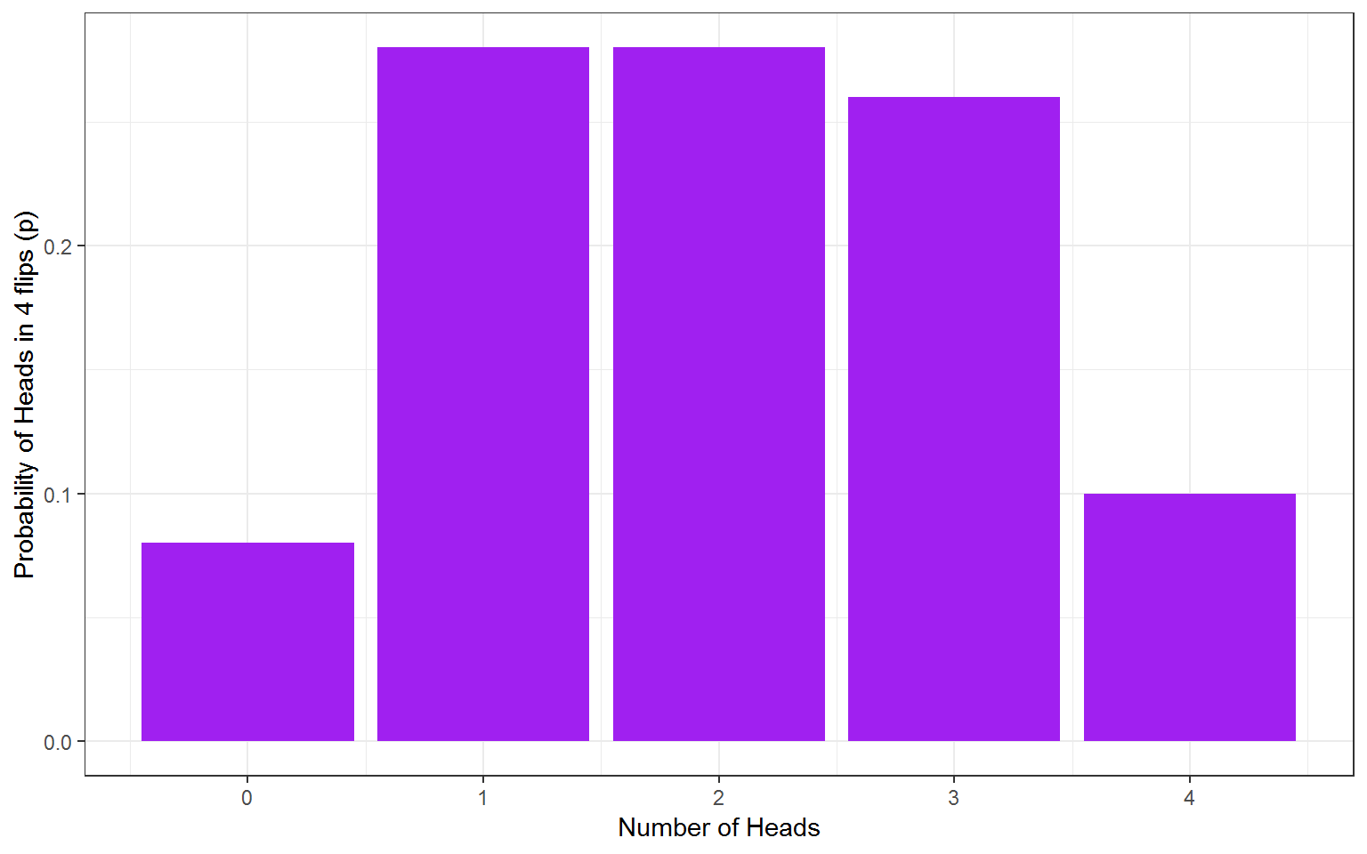
Figure 7.1: No. of heads from 4 coin tosses probability outcomes.
So the estimated probabilites are 0.12 for 0/4 heads, 0.32 for 1/4 heads, etc. Unfortunately sometimes this calculation will estimate that the probabilty of an outcome is zero since this outcome never came up when the simulation is run. If you want reliable estimates, you need a bigger sample as we know that this was a possible outcome but just didnt occur this time.
7.1.14 Activity 9: big data
Let’s repeat the Monte Carlo simulation, but with 10,000 experiments instead of just 50. Here we are again using R to tackle big data and multiple calculations which is much faster and more efficient than if we had to figure this out by hand!
All we have to do is change the 50 to 10000 in the above call to replicate. Again, we’ll put the vector in a tibble and calculate counts and probabilities of each outcome using group_by() and summarise().
heads10K <- replicate(10000, sample(0:1, 4, TRUE) %>% sum())
# this time we save the output in the variable heads10KRemember to try reading your code in full sentences to help you understand what multiple lines of code connected by pipes are doing. How would you read the above code?
ggplot(data10K, aes(heads,p)) +
  geom_bar(stat = "identity", fill = "purple") +
labs(x = "Number of Heads", y = "Probability of Heads in 4 flips (p)") 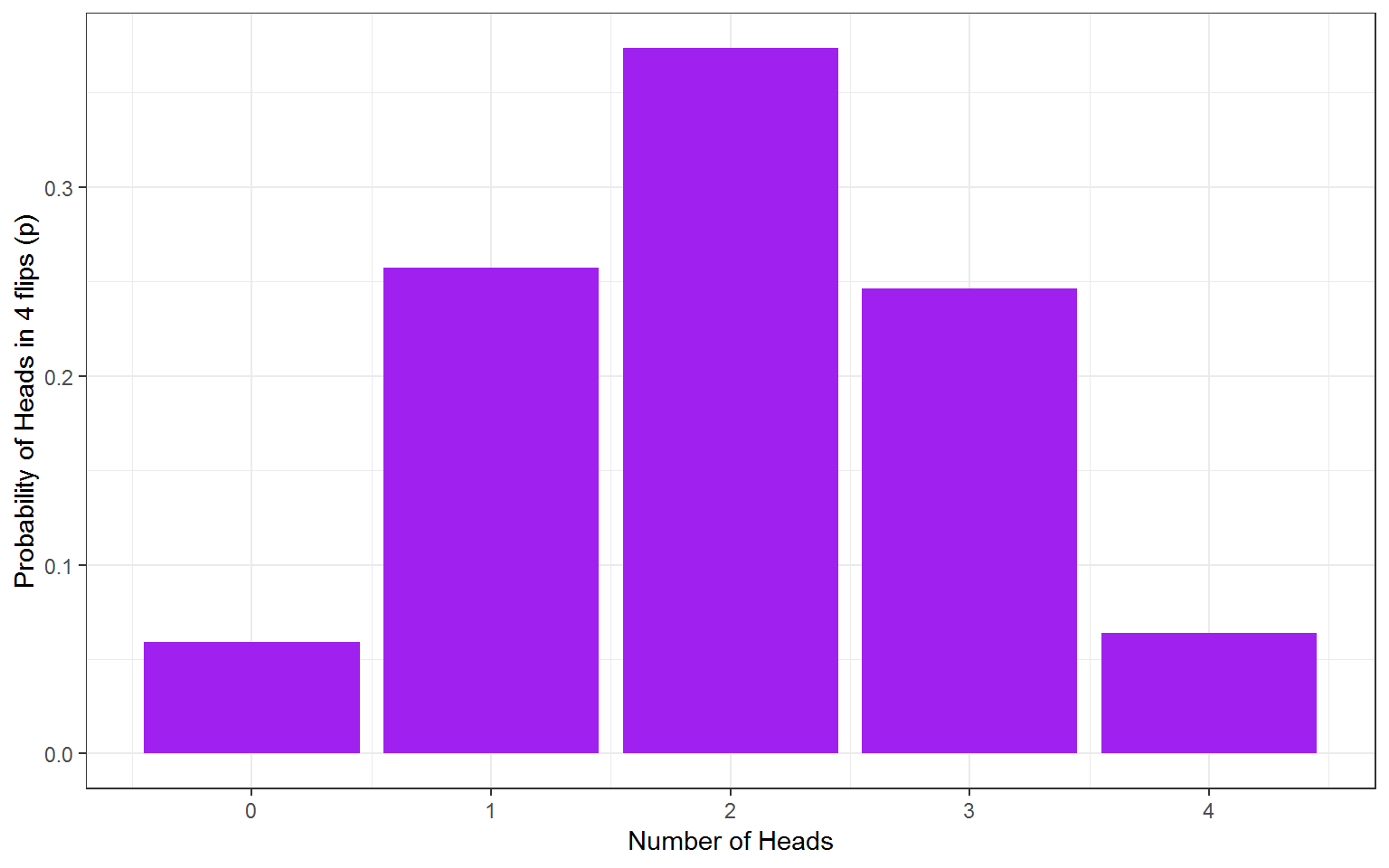
Figure 7.2: 10K coin toss probability outcomes.
Using Monte Carlo simulation, we estimate that the probability of getting exactly one head on four throws is about 0.25. The above result represents a probability distribution for all the possible outcomes in our experiments. We can derive lots of useful information from this.
For instance, what is the probability of getting two or more heads in four throws? This is easy: the outcomes meeting the criterion are 2, 3, or 4 heads. We can just add these probabilities together like so:
## # A tibble: 1 x 1
##      p2
##   <dbl>
## 1 0.684
You can add probabilities for various outcomes together as long as the outcomes are mutually exclusive, that is, when one outcome occurs, the others can’t occur. For this coin flipping example, this is obviously the case: you can’t simultaneously get exactly two and exactly three heads as the outcome of a single experiment. However, be aware that you can’t simply add probabilities together when the events in question are not mutually exclusive: for example, the probability of the coin landing heads up, and it landing with the image of the head being in a particular orientation are not mutually exclusive, and can’t be simply added together.
Additionally, the probabilities we get from Monte Carlo simulations are just estimates; we need something more definitive.
7.1.15 Theoretical probability distributions
Recall that probability is not much more sophisticated than counting and dividing. We are now going to move this forward by looking at binomial distributions in lab 7 and normal distributions in lab 8. See you in lab 7!
\[p = \frac{number \ of \ ways \ the \ event \ could \ arise}{number \ of \ possible \ outcomes}\]
7.2 In-class activities
7.2.1 Monte Carlo simulations
Before we move on, make sure you are comfortable with Monte Carlo simulations that we learnt about in the prep materials. Remember, the staff and GTAs are in the lab to support your learning so if in doubt, just ask one of them to go through it with you. These are concepts that need some work and repetition, so take the time to get comfortable with them as that will put you in good stead moving forward with this lab and lab 4.
7.2.2 The Binomial Distribution - Creating a Discrete Distribution
So far we have learnt how probabilities and distributions work using the simple probability calculation. However, if we wanted to calculate the probability of 8 heads from 10 coin flips we don’t have to go through this entire procedure each time. Instead, because we have a dichotomous outcome, heads or tails, we can calculate probabilities using the binomial distribution - effectively what you just created. We will walk through some essentials here.
We’ll use 3 functions to work with the binomial distribution:
dbinom() - the density function: gives you the probability of x successes given the number of trials and the probability of success on a single trial (e.g., what’s the probability of flipping 8/10 heads with a fair coin?).
pbinom() - the distribution function: gives you the cumulative probability of getting a number of successes below a certain cut-off point (e.g. probability of getting 0 to 5 heads out of 10 flips), given the size and the probability. This is known as the cumulative probability distribution function or the cumulative density function.
qbinom() - the quantile function: is the inverse of pbinom in that it gives you the x axis value below (and including the value) which the summation of probabilities is greater than or equal to a given probability p, plus given the size and prob.
So let’s try these functions out to answer two questions:
- What is the probability of getting exactly 5 heads on 10 flips?
- What is the probability of getting at most 2 heads on 10 flips?
7.2.3 Activity 1: dbinom
Let’s start with question 1, what is the probability of getting exactly 5 heads on 10 flips? We want to predict the probability of getting 5 heads in 10 trials (coin flips) and the probability of success is 0.5 (it’ll either be heads or tails so you have a 50/50 chance which we write as 0.5).
We write that as:
## [1] 0.2460938The probability of getting 5 heads out of 10 coin flips is 0.25 (to 2 decimal places).
which would look like this:
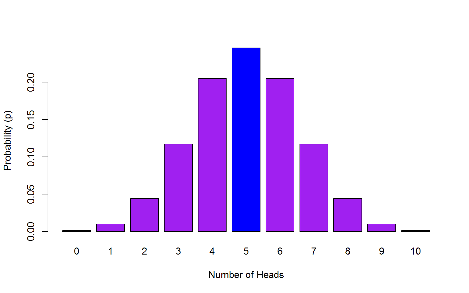
Figure 7.3: 5 heads out of 10 coin toss probability outcomes.
The dbinom (density binom) function takes the format of dbinom(x, size, prob), where the arguments we give are:
*x the number of ‘heads’ we want to know the probability of. Either a single one, 3 or a series 0:10. In this case it’s 5.
*size the number of trials (flips) we are doing; in this case, 10 flips.
*prob the probability of ‘heads’ on one trial. Here chance is 50-50 which as a probability we state as 0.5 or .5
7.2.4 Activity 2: pbinom
OK, question number 2….What is the probability of getting at most 2 heads on 10 flips? This time we use pbinom as we want to know the cumulative probability of getting a maximum of 2 heads from 10 coin flips so we have set a cut-off point of 2 but we still have a probability of getting a heads of 0.5.
- note that the argument name is
qrather thanx. This is because in dbinomxwas a fixed number, whereasqis all the possibilities up to 2 (.e.,g 0, 1, 2).
## [1] 0.0546875The probability of us getting a maximum of 2 heads on 10 coin flips is 0.05 (2 decimal places).
Note that there is another way we could have done this:
## [1] 0.0009765625 0.0107421875 0.0546875000## [1] 0.06640625Note that in this latter strategy, q = 0:2 will give us the probabilties for 0, 1, and 2 heads separately and then we just add these up to calculate the cumulative probablity of this scenario.
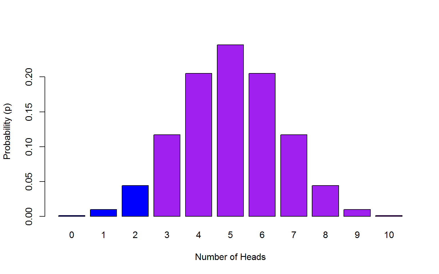
Figure 7.4: Max of 2 heads from 10 coin toss probability outcomes.
Let’s try one more scenario with a cut-off point to make sure we have understood this. What is the probability of getting 7 or more heads on 10 flips? We can actually approach this in two different ways. We have done one way to answer the previous question which we can use again here but instead of using a maximum of 2 coin flips (0:2) we are setting the cut-off as 7 to 10 (7:10).
## [1] 3.933594This doesn’t look quite right does it? Probabilities should be between 0 and 1 not 3.93. The default behaviour of pbinom is to tell us the probability of getting that number of flips or lower. That is, we have summed the probability of getting fewer than 7 heads, fewer than 8 heads, and so on, which is not what we wanted. We can also think about this in terms of the tails of the plots. Are we interested in the lower tail of the plot or the higher tail? The total area under the curve for a theoretical distribution sums to 1. The default behaviour for pbinom is to give us the cumulative probablity of the lower tail - if we want the upper tail instead, we set lower.tail to FALSE, and this will give us the probability for the blue bars.
In this example, we will set lower.tail = FALSE as we are interested in the upper tail of the distribution. Because we want the cumulative probability to include 7, we set q = 6.
## [1] 0.171875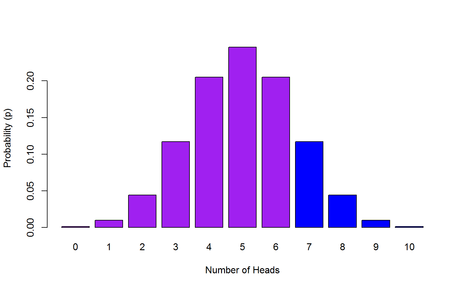
Figure 7.5: Minimum of 7 heads out of 10 coin toss probability outcomes.
7.2.5 Activity 3: qbinom
OK, now let’s consider a scenario in which you’d use the quantile function qbinom. You suspect that the coin is biased against heads. Your null hypothesis is that the coin is not biased against heads (P(heads)=.5). You are going to run a single experiment to test your hypothesis, with 10 trials. What is the minimum number of successes that is acceptable if you want to keep your chances of getting heads for this type of experiment at .05?
You have used the argument prob in the previous two functions, dbinom and pbinom, and it represents the probability of success on a single trial (here it is the probability of ‘heads’ in one coin flip, .5). For qbinom, prob still represents the probability of success in one trial, whereas p represents the overall probability of success across all trials. When you run pbinom, it calculates the number of heads that would give that probability.
In other words, you ask it for the minimum number of successes (e.g. heads) to maintain an overall probability of .05, in 10 flips, when the probability of a success on any one flip is .5.
## [1] 2And it tells you the answer is 2. qbinom also uses the lower.tail argument and it works in a similar fashion to pbinom.
So if you got fewer than two heads, you would reject the null hypothesis that the coin was unbiased against heads.
Ten trials is probably far too few. What would your cutoff be if you ran 100 trials? 1000? 10000?
## [1] 42 474 4918Congratulations! You are well on you way to understanding binomial probability so complete the assessment for this lab and submit one week from attending by 12pm. Next time we will be looking at normal distributions and probability.